Resume Categorization made Easy with NLP and Machine Learning
Learn Data Cleaning, Feature Extraction through TF-IDF and Machine Learning Algorithms

Introduction
The amalgamation of NLP, a branch of artificial intelligence that enables computers to understand, interpret, and generate human-like text, and machine learning algorithms that empower systems to learn patterns from data, creates a foundation for a robust system capable of intelligently categorizing resumes.
One of the cornerstones of this project was the implementation of Term Frequency-Inverse Document Frequency (TF-IDF), a technique that assigns weights to words based on their importance in a document relative to a larger corpus. This allowed for a nuanced analysis of resume content, extracting the essence of skills and qualifications relevant to specific departments.
To further enhance the accuracy and efficiency of the categorization process, I integrated three powerful machine learning models: Support Vector Machines (SVM), Naive Bayes, and K-Nearest Neighbors (KNN). These models, each with its unique strengths, were trained to discern the subtle nuances in language and context, enabling the system to categorize resumes with a high degree of precision.
This blog delves into the step by step process of integrating these technologies to reform the recruitment process and make life much easier for the HR department!
Loading the Dataset
The dataset was obtained from Kaggle, if you want to use the same dataset you can click here.
Since the dataset was in .csv format you can directly load it on Jupyter Notebooks via pandas.
import pandas as pd
df = pd.read_csv(r"Ali Vijdaan\Project NLP\Resume Screening.csv")
df.head()
The output would be a Data Frame like this:
| Category | Resume | |
| 0 | Data Science | Skills * Programming Languages: Python (pandas... |
| 1 | Data Science | Education Details \r\nMay 2013 to May 2017 B.E... |
| 2 | Data Science | Areas of Interest Deep Learning, Control Syste... |
| 3 | Data Science | Skills ⢠R ⢠Python ⢠SAP HANA ⢠Table... |
| 4 | Data Science | Education Details \r\n MCA YMCAUST, Faridab... |
At this point you might be confused about the random signs and characters included under the Resume column, however, don't worry we would be cleaning the data later on.
Data Pre-processing
Ah! The backstage cleanup crew of the data world – data preprocessing! Let me walk you through the steps.
Spotting the Empty Seats
If the dataset were to be a large party, then the null values would be the empty seats. First things first, we need to identify those empty chairs.
 rows, col = df.shape
 print(f"Rows: {rows}")
 print(f"Columns: {col}")

 null_sum = df.isnull().sum()
 print(null_sum)
The following code allows us to find the total rows and column of the dataset plus the total number of null values.
Say Goodbye to Outliers
Outliers are like party crashers - they mess up the whole vibe. Lets make a function a to give the party crashers a send away.
import re
import nltk
from gensim.parsing.preprocessing import remove_stopwords
from nltk.stem import WordNetLemmatizer

#Creating instance
lemmatizer = WordNetLemmatizer()

def dataCleaning(txt):
    CleanData = re.sub('https\S+\s', ' ', txt)  #Cleaning links via re
    CleanData = re.sub(r'\d', ' ', CleanData)   #Cleaning numbers via re
    CleanData = re.sub('@\S+', ' ', CleanData)  #Cleaning email address via re
    CleanData = re.sub('#\S+\s', ' ', CleanData)    #Cleaning # symbol via re
    CleanData = re.sub('[^a-zA-Z0-9]', ' ', CleanData)  #Cleaning special characters via re
    CleanData = remove_stopwords(CleanData) #Cleaning stopwords via genism
    CleanData = lemmatizer.lemmatize(CleanData) #Lemmatization via nltk
    return CleanData
Lets break down the code to understand it easier. We use nltk, re and genism to clean the data. The function first includes re to clean links, numbers, emails addresses, and special characters.
Then we remove stop words. Stop words are words like 'the', 'on', 'to', etc. which are removed to reduce the size of the corpus.
Lastly we apply lemmatization.
Lemmatization
It links similar meaning words as one word, making tools such as chatbots and search engine queries more effective and accurate. For example, 'walking', 'walked' or 'walks' will be converted to 'walk'.
For lemmatization we use WordNetLemmatizer, however, for this to work we have to download the wordnet dataset.
nltk.download('wordnet')
After constructing the function, lets apply it on our data frame.
df['Resume'] = df['Resume'].apply(lambda x : dataCleaning(x))
Label Encoding
The questions arises - what's the need for labelling the different categories? Well, it would be much easier for the computer to match a certain number with a specific type of resume than some string.
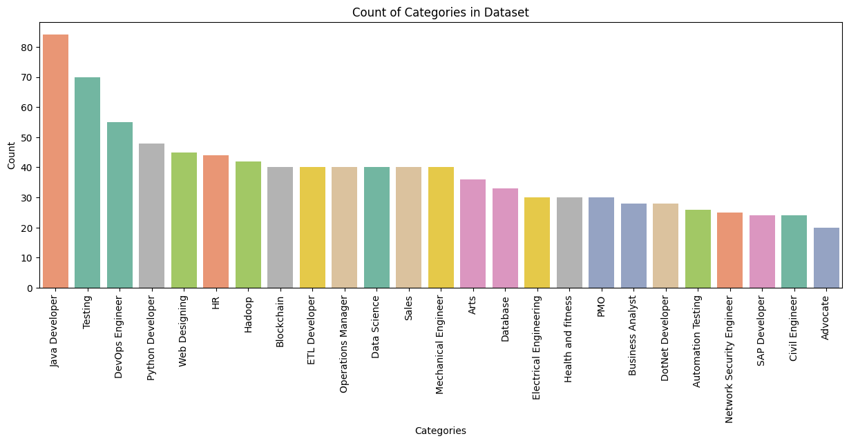
But before that let's analyze the number of categories we have in the first place.
 import seaborn as sns

 plt.figure(figsize = (15, 5))
 sns.countplot(x='Category', data = df, order = df['Category'].value_counts().index, palette='Set2', hue = 'Category')
 plt.xticks(rotation = 90)
 plt.ylabel('Count')
 plt.xlabel('Categories')
 plt.title('Count of Categories in Dataset')
 plt.show()
The above code makes a simple count plot using
seabornof the different categories. It uses.value_counts()from thepandaslibrary to count the size per library.This is what the plot looks like.
Now lets give these categories their labels!
 from sklearn.preprocessing import LabelEncoder

 le = LabelEncoder()

 le.fit(df['Category'])
 df['Labeled Category'] = le.transform(df['Category'])

 print(df[['Category', 'Labeled Category']])
What we did here was use the
sklearn.preprocessingmodule to import theLabelEncoderclass which specifically used for label encoding.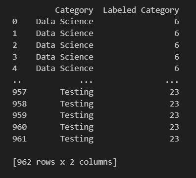
Feature Extraction
Feature extraction involves converting raw data, in this case, text from resumes, into a format suitable for machine learning algorithms. It's the process of distilling relevant information from the data, creating a condensed representation that captures the essence of the original content.
While TF-IDF is our protagonist today, it's not the lone ranger in the feature extraction arena. Other techniques include:
Bag-of-Words (BoW): Counts the frequency of each word in a document, disregarding order.
Word Embeddings (e.g., Word2Vec, GloVe): Represents words as dense vectors, capturing semantic relationships.
Doc2Vec (Paragraph Vector): Extends word embeddings to represent entire documents.
Latent Semantic Analysis (LSA): Applies singular value decomposition to discover hidden relationships between terms.
What is TF-IDF?
TF-IDF, or Term Frequency-Inverse Document Frequency, is a numerical statistic that reflects the importance of a word in a document relative to a collection of documents (corpus). It balances the frequency of a term (TF) with its rarity across documents (IDF), emphasizing terms that are specific to a document while downplaying common words.
from sklearn.feature_extraction.text import TfidfVectorizer

tfidf = TfidfVectorizer()

tfidf.fit(df['Resume'])
requiredText = tfidf.transform(df['Resume'])
In summary, this code snippet sets up and utilizes the TfidfVectorizer to transform the textual content of resumes into a numerical format, allowing for further analysis and modeling. The resulting requiredText matrix serves as a feature representation that can be used in machine learning tasks, capturing the importance of words in each resume relative to the entire collection.
Splitting the Data
By splitting the dataset, you can train your machine learning model on one subset and evaluate its performance on another. This helps assess how well the model generalizes to new, unseen data.
from sklearn.model_selection import train_test_split

x_train, x_test, y_train, y_test = train_test_split(requiredText, df['Labeled Category'], test_size = 0.3, random_state = 42)

train_row, train_col = x_train.shape
test_row, test_col = x_test.shape

print(f"Training data Rows: {train_row}")
print(f"Training data Columns: {train_col}")
print(f"Testing data Rows: {test_row}")
print(f"Testing data Columns: {test_col}")
The train_test_split function takes two main arguments: the features (requiredText) and the target variable (df['Labeled Category']). It also specifies the test size (in this case, 30% of the data is reserved for testing) and a random state for reproducibility (random_state=42).
The result is four sets of data: x_train (features for training), x_test (features for testing), y_train (target variable for training), and y_test (target variable for testing).
Machine Learning Algorithms
Now that we have our data neatly split into training and testing sets, the stage is set for the real magic – integrating machine learning algorithms. This step involves training a model on the training dataset and then evaluating its performance on the testing dataset to ensure it can generalize well to new, unseen data.
k-Nearest Neighbor
k-Nearest Neighbors is a simple yet powerful algorithm used for both classification and regression tasks. The fundamental idea is to predict the label of a data point by looking at the 'k' closest data points in the feature space. In other words, it makes predictions based on the majority class or average value of its nearest neighbors.
from sklearn.multiclass import OneVsRestClassifier
from sklearn.neighbors import KNeighborsClassifier

clf = OneVsRestClassifier(KNeighborsClassifier())
clf.fit(x_train, y_train)
ypred_knn = clf.predict(x_test)
print(ypred_knn)
The One-vs-Rest Classifier is employed to extend the KNN algorithm for multi-class classification tasks. It essentially transforms a multi-class problem into a series of binary classification problems (one for each class).
In essence, the code snippet demonstrates the application of the k-Nearest Neighbors algorithm within a multi-class classification framework using the One-vs-Rest strategy. This approach is particularly useful when dealing with problems where instances may belong to multiple classes simultaneously.
Multinomial Naive Bayes
The Multinomial Naive Bayes variant is specifically designed for text classification problems, where the features are often word counts or term frequencies. It's commonly used when dealing with discrete data, making it well-suited for tasks like document classification or, in this case, categorizing resumes based on their content.
from sklearn.naive_bayes import MultinomialNB

model = OneVsRestClassifier(MultinomialNB())
model.fit(x_train, y_train)
ypred_nb = model.predict(x_test)
print(ypred_nb)
The code follows the same pattern as with KNN we did above.
Support Vector Machine
Imagine you have data points of two different classes on a graph. SVM helps find the best possible line (hyperplane) that creates the maximum separation between these classes. This line is like a referee trying to keep players from two teams as far apart as possible. The farther apart, the more confident we can be about the classification.
from sklearn.svm import SVC

model_svm = OneVsRestClassifier(SVC())
model_svm.fit(x_train, y_train)
ypred_svm = model_svm.predict(x_test)
print(ypred_svm)
Comparative Analysis
Comparative analysis among machine learning algorithms is like hosting a talent show for models – you want to find the superstar that steals the spotlight! Just like judging a dance-off, we evaluate metrics like accuracy, precision, and recall to determine who's got the smoothest moves in predicting resume categories. It's not just about picking a winner; it's about understanding which algorithm suits the rhythm of your data, ensuring the ultimate ensemble of models that can boogie through the complexities of your task with flair!
knn_accuracy = clf.score(x_test, y_test) * 100
nb_accuracy = model.score(x_test, y_test) * 100
svm_accuracy = model_svm.score(x_test, y_test) * 100

ml_models = ['KNN', 'Naive Bayes', 'SVM']
ml_perc = [ knn_accuracy, nb_accuracy, svm_accuracy]

plt.figure(figsize=(8, 6))
bars = plt.bar(ml_models, ml_perc, color='skyblue')
plt.xlabel('Machine Learning Models')
plt.ylabel('Percentage')
plt.title('Accuracy Percentage of Different Models')
plt.ylim(0, 100)

for bar, ml_perc in zip(bars, ml_perc):
    plt.text(bar.get_x() + bar.get_width() / 2, bar.get_height() - 5, f'{round(ml_perc, 2)}%', ha='center', va='bottom', fontsize=10, color='black')

plt.show()
This code calculates and visualizes the accuracy percentages of three machine learning models (K-Nearest Neighbors, Naive Bayes, and Support Vector Machine) in a fun bar chart. The accuracy scores for each model on the testing dataset are represented by bars, with labeled percentages atop each bar. It offers a quick and visual snapshot of how well each model performs in categorizing resumes into different departments.
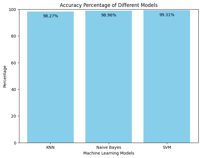
The high accuracy scores suggest that all three machine learning models (SVM, Naive Bayes, and KNN) are performing remarkably well in categorizing resumes.
Furthermore, we see that SVM has the greatest accuracy!
The reasons why Support Vector Machines (SVM) achieved the highest accuracy might be due to several reasons:
Complex Decision Boundaries: SVM excels in capturing intricate relationships in the data due to its ability to create complex decision boundaries.
Effective in High-Dimensional Spaces: SVM's performance is notable in datasets with a large number of features, common in text-based applications like resume categorization.
Handling Outliers: SVM's insensitivity to outliers contributes to its stability in the presence of data points that deviate from the general pattern.
With the accuracy noted, lets delve deeper into the analysis about each individual algorithm. A good way to do that is to create a simple classification report.
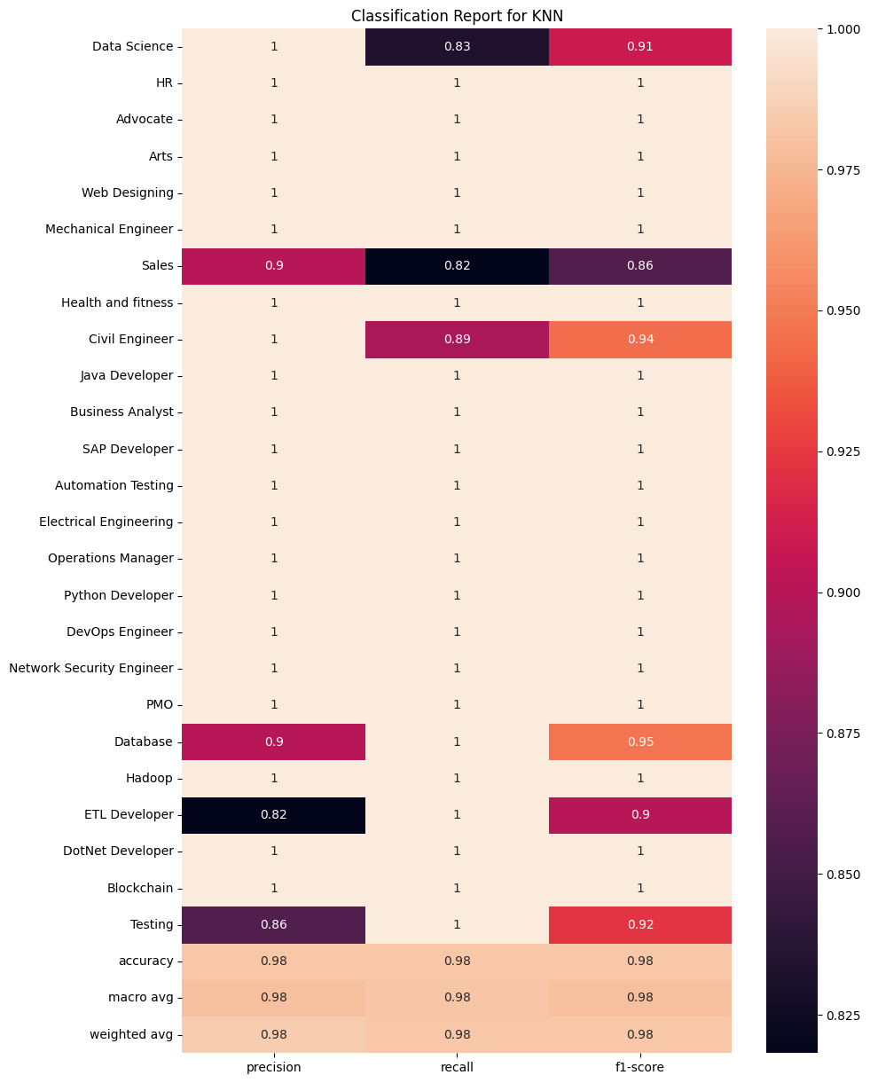
k-Nearest Neighbor
from sklearn.metrics import classification_report

clf_report = classification_report(y_test, ypred_knn, target_names = df['Category'].unique(), output_dict=True)
plt.figure(figsize=(10, 15))
sns.heatmap(pd.DataFrame(clf_report).iloc[:-1, :].T, annot=True)

plt.title('Classification Report for KNN')
plt.show()
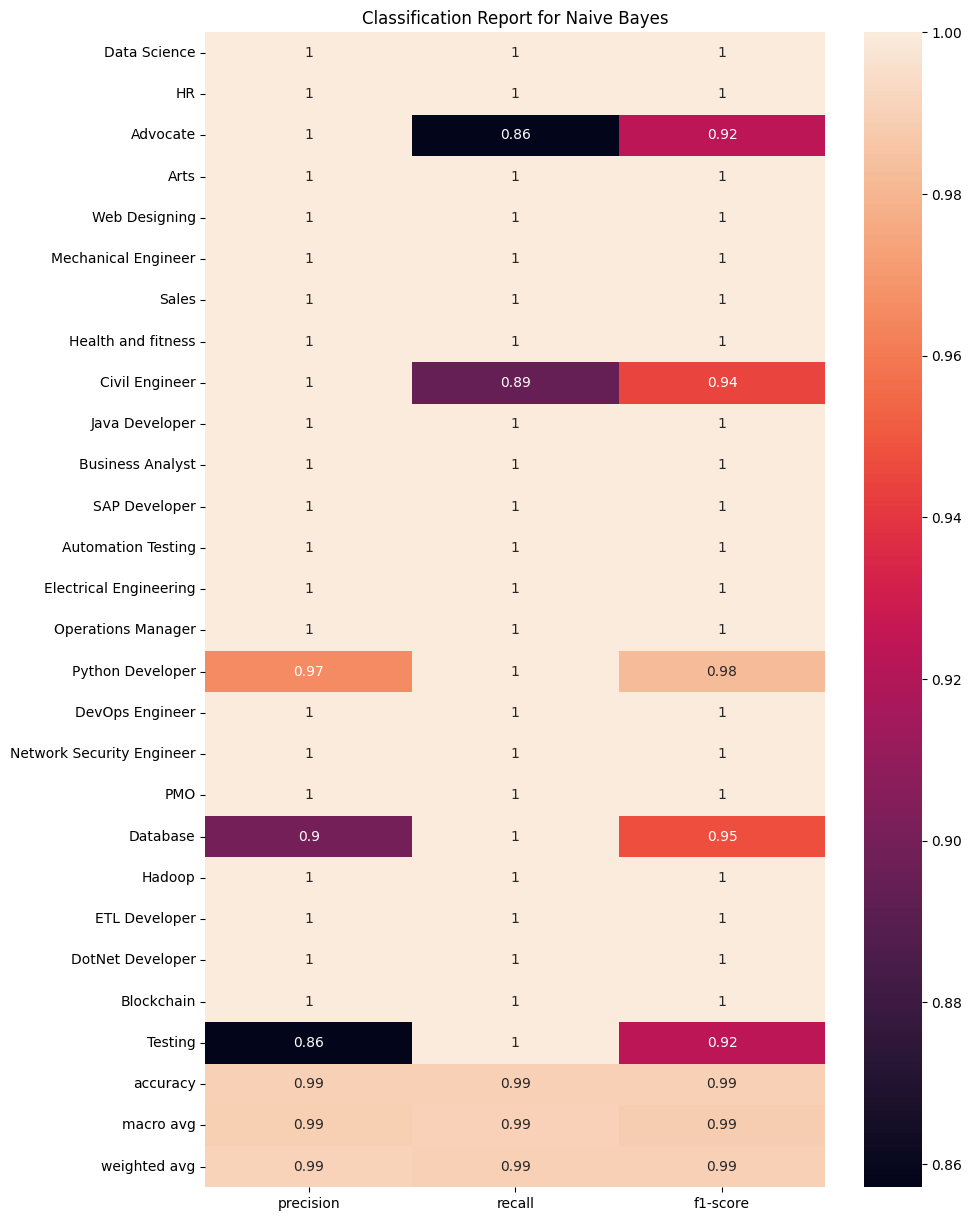
Multinomial Naive Bayes
clf_report = classification_report(y_test, ypred_nb, target_names = df['Category'].unique(), output_dict=True)
plt.figure(figsize=(10, 15))
sns.heatmap(pd.DataFrame(clf_report).iloc[:-1, :].T, annot=True)

plt.title('Classification Report for Naive Bayes')
plt.show()
Support Vector Machines
clf_report = classification_report(y_test, ypred_svm, target_names = df['Category'].unique(), output_dict=True)
plt.figure(figsize=(10, 15))
sns.heatmap(pd.DataFrame(clf_report).iloc[:-1, :].T, annot=True)

plt.title('Classification Report for SVM')
plt.show()
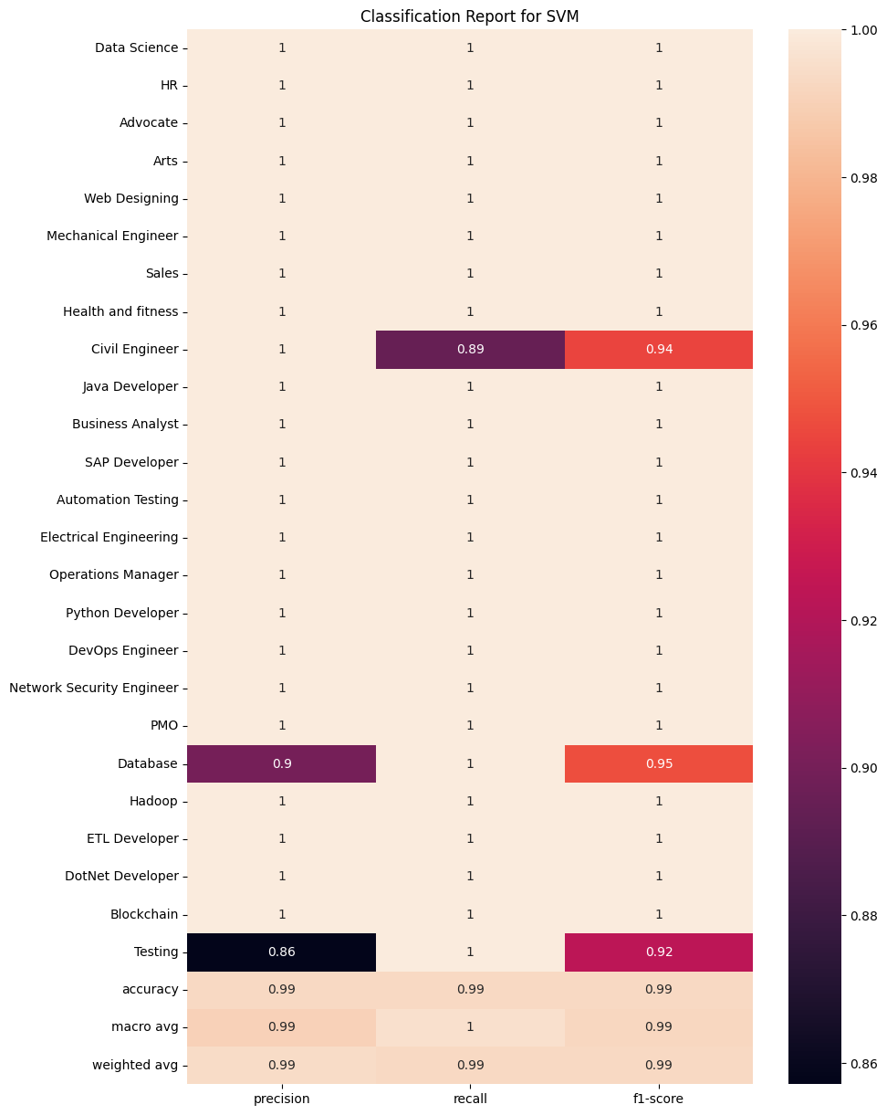
These heatmaps show further information through the precision, recall and f1-score of each individual algorithm.
If you want to read the entire code along with how I integrated this project into a prediction system via pickle then click here.
print("Happy Coding!)


